Category: MATLAB

Solving Systems of Differential Equations with MATLAB
A system of differential equations contain two or more equations that are related by two dependent variables that share a single common independent variable like t for time. Applications of systems of differential equations range from engineering, science, and applied mathematics.

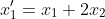
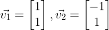
Consider the following system of differential equations:

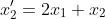
First, we manually solve for a general solution of the system, then we use MATLAB to come up with a solution.

Solving for a General Solution Manually

The first step is to create a coefficient matrix of the system, then solve for the eigenvalues and associated eigenvectors.

The coefficient matrix for the system is the following:

Next, the eigenvalues are solved for, which means solve for the determinant, and set it equal to zero:

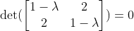
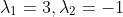
By solving this, you will obtain the following eigenvalues:

Now that we have the eigenvalues, we can solve for the associated eigenvectors. This can be done by solving the following for each eigenvalue:

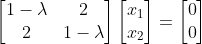
Doing so, we obtain the following associated eigenvectors:

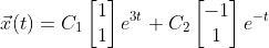
Therefore, the general solution will be the following:

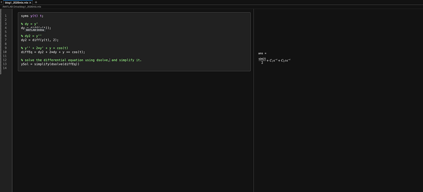
Solving For a General Solution with MATLAB

First, let’s solve for the eigenvectors and eigenvalues using MATLAB. The following code will do that.
```
% Coefficient matrix 
A = [1 2; 2 1];

% Solve for eigenvalues D and eigenvectors V
[V,D] = eig(A);

% Get the first eigenvector and scale
eigV1 = V(:,1) ./ min(V(:,1))

% Get the second eigenvector and scale
eigV2 = V(:,2) ./ min(V(:,2))

x1Vec = -1:0.05:1;
x2Vec = -1:0.05:1;

% x2 = -x1
v1 = -1*x1Vec;
% x2 = x1
v2 = x1Vec;

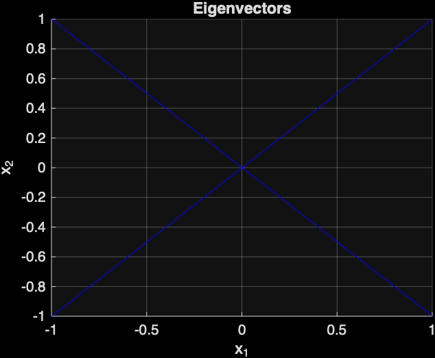
% Plot the eigenvectors
figure;
hold on;
plot(x1Vec,v1,'b');
plot(x1Vec,v2,'b');
xlabel('x_{1}');
ylabel('x_{2}');
grid on;

title('Eigenvectors');
% put the axes on the same limits
xlim([-1 1]);
ylim([-1 1]);
```
The following is the plot that was generated by MATLAB of the two eigenvectors:

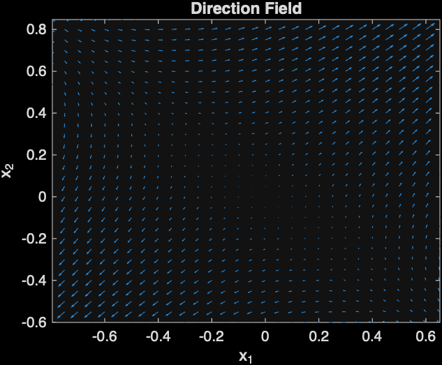
Next, let’s plot the direction field, which will show the direction of solution curves with respect to time.

The following MATLAB code will do that:
```
[x1, x2] = meshgrid(x1Vec,x2Vec);
% Compute the direction field at the grid of points
x1dot = x1 + 2*x2;
x2dot = 2*x1 + x2;

% The quiver command can be used to plot the direction field
figure;
quiver(x1,x2,x1dot, x2dot);
xlabel('x_{1}');
ylabel('x_{2}');
title('Direction Field');
xlim([-1 1]);
ylim([-1 1]);
```
The following direction field was generated by MATLAB:

Next, a phase portrait will be generated with MATLAB, which will show the relationship between x1 and x2 with respect to time. The arrows shows the point on a particular solution curve with respect to time.
```
figure;
streamslice(x1Vec,x2Vec,x1dot,x2dot);
title('Phase Portrait');
```
The following is the plot that was generated:

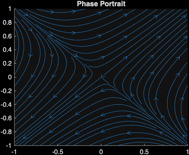
This image indicates that the point (0,0) is a saddle point. Also, you can tell that the graph will be a saddle because the eigenvalues are both real and one is positive and the other is negative.

Final Words

You saw an example of solving a system of differential equations, and you learned how to solve it using MATLAB.
May 13, 2026
Katherine Johnson and Numerically Approximating a Solution to a Differential Equation with Euler’s Method using MATLAB
Euler’s method is used for numerical approximation of a solution to a differential equation that can’t be solved for an explicit solution using elementary methods, such as substitution for homogeneous equations or Bernoulli equations (Henry Edwards et al., 2022). Katherine Johnson used Euler’s method to solve real-world problems at NASA (Meyers, 2017). Personally, I disagree with her claim that math is either absolutely right or absolutely wrong, though.

The algorithm for Euler’s method is to first pick an initial point

of the particular solution you want to compute (Henry Edwards et al., 2022). Then, one chooses a horizontal step-size h, which is the horizontal distance between the approximated points of the solution. The formula to calculate the (n+1)-th point is the following (Henry Edwards et al., 2022):

where

One must be careful when using Euler’s method because there is a local error when moving away from the initial point, which is a vertical distance from the approximated point to the actual point of the particular solution curve (Henry Edwards et al., 2022). As one moves further from the initial point, the error accumulates, and it is called cumulative error (Henry Edwards et al., 2022). The remedy for this is to choose a sufficiently small step size, which will reduce the error (Henry Edwards et al., 2022). However, there is typically a tradeoff when picking h because when h is too small, it may take thousands of years to compute even with a computer (Henry Edwards et al., 2022).

Katherine Johnson was an African American applied mathematician who worked at NASA (Meyers, 2017). She suggested to use Euler’s method to solve differential equations related to the trajectory of astronaut John Glenn’s space capsule. Despite the method being “ancient”, as described by one of her male colleagues, she rebutted that “it works numerically” (Meyers, 2017).

When Katherine Johnson claims “math: you’re either right or wrong — and that I liked about it” (National Geographic, 2021, 0:45) , I tend to disagree. I disagree because sometimes oversimplified models can enable one to capture important insights into the problem. For example, the Lotka-Volterra predator-prey model allows one to see that predator-prey populations oscillate; however, the models typically do not allow one to actually predict the populations in nature (Chasnov, 2022; Clark & Neuhauser, 2022). This is a case in mathematics where it is possible to be partially correct.

In conclusion, Euler’s method is an old yet effective way to numerically approximate solutions to differential equations. It has been used to solve real-world problems in NASA by applied mathematicians like Katherine Johnson to calculate trajectories of a space capsule. Also, despite Katherine Johnson’s claim that one is either right or wrong in math, I think that it is possible to be partially correct in math in the case of oversimplified models that allow one to gain further insights into problems like the Lotka-Volterra predator-prey model.

Using MATLAB to Obtain a Numerical Approximation of a Solution

Next, MATLAB will be used to solve the following differential equation:

with initial condition y(0) = -3.

The following is the MATLAB code to do so:
```
% Euler's Method for solving:
% y' = x + (1/5)y
% y(0) = -3

clc;
clear;

% Step size
h = 1;

% Interval
x0 = 0;
xn = 5;

% Initial condition
y0 = -3;

% Number of steps
n = (xn - x0)/h;

% Arrays to store values
x = zeros(1, n+1);
y = zeros(1, n+1);

% Initial values
x(1) = x0;
y(1) = y0;

% Euler's Method loop
for i = 1:n
    x(i+1) = x(i) + h;
    y(i+1) = y(i) + h * ( x(i) + (1/5)*y(i) );
end

% Display results
disp('   x          y');
disp([x' y']);

% Plot the approximation
plot(x, y, '-', 'LineWidth', 1.5);
xlabel('x');
ylabel('y');
title('Euler Method Approximation');
grid on;
```
References

Chasnov, J. R. (2022, January 5). 1.4: The Lotka-Volterra predator-prey model. Mathematics LibreTexts; Libretexts. https://math.libretexts.org/Bookshelves/Applied_Mathematics/Mathematical_Biology_%28Chasnov%29/01%3A_Population_Dynamics/1.04%3A_The_Lotka-Volterra_Predator-Prey_Model

Clark, A. T., & Neuhauser, C. (2018). Harnessing uncertainty to approximate mechanistic models of interspecific interactions. Theoretical Population Biology, 123, 35–44. https://doi.org/10.1016/j.tpb.2018.05.002

Henry Edwards, C., Penney, D. E., & Calvis., D. (2022). Differential Equations and Boundary Value Problems: Computing and Modeling (6th Edition).

Meyers, C. (2017, February 24). Exploring the math in “hidden figures.” AIP. https://www.aip.org/inside-science/exploring-the-math-in-hidden-figures
May 13, 2026
Solving Differential Equations with MATLAB
Differential equations show up everywhere in science and engineering: vibrating springs, electrical circuits, population models, and control systems all rely on them. In this post, we’ll walk through how to solve the second-order linear differential equation

y′′+2y′+y=cos⁡(t)

Afterwards, it will be demonstrated how to solve such a problem with MATLAB.

Solve the Homogeneous Equation

We begin with the associated homogeneous equation:

y′′+2y′+y=0

To solve it, we use the characteristic equation method. Replace:
- y′′→r²
- y′→r
- y→1
This gives:

r²+2r+1=0

Factor the polynomial:

(r+1)²=0

So we have a repeated root:

r=−1

For a repeated root r, the homogeneous solution is:

where C1 and C2 are arbitrary constants.

Find a Particular Solution

Now we need a particular solution y_p(t) to account for the forcing term cos⁡(t).

Because the right-hand side is trigonometric, we try:

y_p(t)=Acos⁡(t)+Bsin⁡(t)

Differentiate:

y_p′(t)=−Asin⁡(t)+Bcos⁡(t)

y_p′′(t)=−Acos⁡(t)−Bsin⁡(t)

Substitute these into the differential equation:

y_p′′+2y_p′+y_p=cos(t)

Substituting term by term:

(−Acos⁡(t)−Bsin(⁡t))+2(−Asin⁡(t)+Bcos⁡(t))+(Acos⁡(t)+Bsin⁡(t))=cos(t)

Notice that the Acos⁡(t) and −Acos⁡(t) cancel, and the Bsin(⁡t) terms also cancel:

2Bcos⁡(t)−2Asin⁡(t)=cos(t)

Now match coefficients.

For cos⁡(t):

2B=1

so

B=1/2

For sin(⁡t):

−2A=0

so

A=0

Therefore,

y_p(t)=(1/2)*sin⁡(t)

Write the General Solution

The full solution is the sum of the homogeneous and particular solutions:

So the final answer is

Why This Method Works

This approach is standard for linear differential equations with constant coefficients:
1. Solve the homogeneous equation using the characteristic polynomial.
2. Guess a form for the particular solution based on the forcing term.
3. Determine unknown coefficients by substitution.
4. Combine both parts.
The exponential portion captures the system’s natural behavior, while the sine term reflects the external forcing function.

Solving with MATLAB

The following is the MATLAB code that will solve the problem:
```
syms y(t) t;

% dy = y'
dy = diff(y(t));

% dy2 = y''
dy2 = diff(y(t), 2);

% y'' + 2*y' + y = cos(t)
diffEq = dy2 + 2*dy + y == cos(t);

% solve the differential equation and simplify it.
simplify(dsolve(diffEq))
```
By executing the code, you will obtain the same answer that was manually solved for:

Running the above MATLAB code and obtaining the same solution.

Final Thoughts

The equation

y′′+2y′+y=cos⁡(t)

is a classic example of a damped, driven system. The repeated root in the homogeneous solution creates the factor of te^(−t), while the cosine forcing introduces a sinusoidal steady-state response.

Once you’re comfortable with this process, you can apply it to a huge class of differential equations that appear in physics, engineering, and applied mathematics.
May 12, 2026