In this blog post, you will learn what a Laplace Transform is, and how to use them to solve differential equations.
What is a Laplace Transform?
Laplace Transforms are important because they enable you to solve differential equations algebraically. Therefore, they are important for solving problems in science, engineering, and applied math.
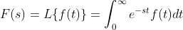
The definition of a Laplace Transform is the following:
Given a function f(t) defined for all t greater than or equal to zero, the Laplace Transform of f is the function F defined as follows:
For all values of s for which the improper integral converges.
Computing the Laplace Transform by Definition
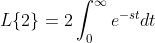
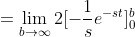
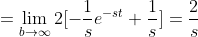
Let’s look at a simple function f(t)=2, and compute its Laplace Transform.
Note: once you compute some of these by hand, you notice you keep using the same ones over and over. Therefore, there are tables of Laplace transforms you can reference to compute them. You can also use them for computing the inverse of the transform.
Inverse Transforms
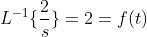
As you might guess, sometimes, we want to reverse F(s) back to a function f(t), which is the inverse Laplace Transform. Since, we just computed one, let’s reverse it.
This is important when you want to transform the algebraically solved expression back into a particular solution of a differential equation (more on that later.)
Solving a Differential Equation with Laplace Transforms
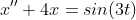
Consider the following differential equation:
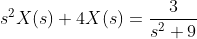
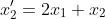
with the initial conditions x(0)=x'(0)=0. Taking the Laplace transform of it converts it into the following:
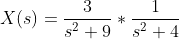
Solving for X(s), we get the following:
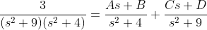
Now, to compute the inverse Laplace transform, which will give us x(t). We must use partial fractions, which gives us the following:
Solving this partial fraction, you will obtain A=C=0, B= 3/5, and D=-3/5.
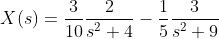
Therefore, we have the following:
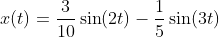
By computing the inverse Laplace transform, we get x(t), which is the following:
This is the particular solution to the equation given the initial conditions.
Final Thoughts
In this blog post, you learned what Laplace transforms are, and you learned how to use them to solve differential equations.
In this blog post, you will learn how to manually calculate and check poker odds.
The Game of Poker
A deck of cards has a total of 52 cards with four suits, which are hearts, diamonds, clubs, and spades. Each suit has 13 card values, which are the numbers 2-10, Jack, Queen, King, Ace. The ace card can act as a high or low value card.
In the game of poker, 5 cards make up a hand. The following diagram shows what type of hands you can get.
Getting a pair, two pair, three of a kind, and four of a kind are pretty straightforward.
A straight is a sequence of cards that are in increasing order, and the cards can be of different suits. The hand must contain each consecutively increasing card value. For example, the cards, 2,3,4,5,6 is a straight, but the cards 2,5,7,9,10 is not a straight.
A flush is a sequence of cards of the same suit. The cards do not need to be consecutively increasing like a straight. For example, the cards 5, 7, 8, 10, K would be a flush.
A full house is a hand with both three of a kind and a pair.
A straight flush is a hand that is both a flush and a straight at the same time.
A royal flush is a hand that contains the values, 10, J, Q, K, A where the ace counts as a high card.
The Odds of Getting a Pair
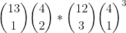
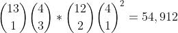
Let’s first go over the theory of receiving a hand with a pair in poker. To count the number of ways, we use a combination of combinatorics and the multiplication rule. The first thing we want to do is choose 1 card value of 13 values. Then choose 2 cards from two different suits. Afterwards, we want to choose 3 different card values from the remaining 12 values, and choose each of the three cards from four different suits. The total number of ways to get a pair is then the following:
This number is 1,098,240. To get the odds, we divide the previous number with the total number of ways to choose 5 cards from a deck of 52 cards. The odds turn out to be 42.2569% to get a pair.
The following is the code to simulate the odds of getting a pair:
import random

class Card():
    def __init__(self, value, suit):
        self._value = value
        self._suit = suit

    def value(self):
        return self._value

    def suit(self):
        return self._suit

    def __str__(self):
        return "" + self._suit + str(self._value)

def create_deck():
    deck = []
    suit = ["H", "D", "S", "C"]

    for i in range(13):
        for j in range(4):
            deck.append(Card(i, suit[j]))

    return deck

def shuffle_deck(deck):
    random.shuffle(deck)

def draw_hand(deck):
    hand = []

    for i in range(5):
        c = deck.pop()
        hand.append(c)

    return hand

def print_hand(hand):
    print("Hand:", end="")
    for c in hand:
        print(c, "", end="")
    print("")

def has_pair(hand):
    # This variable ensures there will be only one
    # pair
    meta_count = 0

    for i in range(5):
        # Count the number of cards with
        # the same value as the i-th card.
        count = 0
        for j in range(i+1, 5):
            if hand[i].value() == hand[j].value():
                count += 1
                continue


        if count == 1:
            meta_count += 1
        elif count == 2:
            return False
        elif count == 3:
            return False

    return meta_count == 1


def main():
    run_count = 100000
    pair_count = 0

    for x in range(run_count):
        deck = create_deck()
        shuffle_deck(deck)
        hand = draw_hand(deck)
        print_hand(hand)

        if has_pair(hand):
            pair_count += 1

    print("Expected Probability: 42.2569%")
    print("Simulated Probability: " + str(pair_count/ 100000.0))

if __name__ == "__main__":
    main()
The Odds of Getting Three of a Kind
The theory for getting three of a kind is as follows:
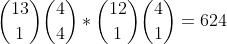
From 13 different values, we want to choose one value, then of four suits we want to choose 3 from 4. Then, from 12 remaining values, we want to choose only two more cards and then choose one card from four suits twice.
The count turns out to be the following:
To get the odds, we divide that number by the total number of ways to choose 5 cards from a deck of 52 cards. This turns out to be 2.11285%
The following is the code to simulate the odds of getting three of a kind:
import random

class Card():
    def __init__(self, value, suit):
        self._value = value
        self._suit = suit

    def value(self):
        return self._value

    def suit(self):
        return self._suit

    def __str__(self):
        return "" + self._suit + str(self._value)

def create_deck():
    deck = []
    suit = ["H", "D", "S", "C"]

    for i in range(13):
        for j in range(4):
            deck.append(Card(i, suit[j]))

    return deck

def shuffle_deck(deck):
    random.shuffle(deck)

def draw_hand(deck):
    hand = []

    for i in range(5):
        c = deck.pop()
        hand.append(c)

    return hand

def print_hand(hand):
    print("Hand:", end="")
    for c in hand:
        print(c, "", end="")
    print("")

def has_pair(hand):
    meta_count = 0
    for i in range(5):
        count = 0
        for j in range(i+1, 5):
            if hand[i].value() == hand[j].value():
                count += 1
                continue


        if count == 1:
            meta_count += 1
        elif count == 2:
            return False
        elif count == 3:
            return False

    return meta_count == 1

def three_of_a_kind(hand):
    count_map = {}

    for c in hand:
        if c.value() not in count_map:
            count_map[c.value()] = 1
        else:
            count_map[c.value()] += 1

    has_two_of_a_kind = False
    has_three_of_a_kind = False

    for k in count_map:
        if count_map[k] == 2:
            has_two_of_a_kind = True
        elif count_map[k] == 3:
            has_three_of_a_kind = True

    return has_three_of_a_kind and not has_two_of_a_kind

def main():
    run_count = 100000
    three_of_a_kind_count = 0

    for x in range(run_count):
        deck = create_deck()
        shuffle_deck(deck)
        hand = draw_hand(deck)
        print_hand(hand)

        if three_of_a_kind(hand):
            three_of_a_kind_count += 1

    print("Simulation Probability: " + str(three_of_a_kind_count/ 100000.0))

if __name__ == "__main__":
    main()
The Odds of Getting Four of a Kind
The theory for getting four of a kind is as follows:
First, we want to choose 1 card value from 13 possible card values. Second, choose all 4 from 4 different suits. Next we want to multiply that with choosing one card value from 12 remaining values, and then multiply that by choosing 1 suit from 4 suits. This turns out to be the following:
To get the odds, we divide 624 by the total number of ways to choose 5 cards from a 52 card deck. This turns out to be 0.024%
The code to simulate the odds of getting four of a kind is the following:
import random

class Card():
    def __init__(self, value, suit):
        self._value = value
        self._suit = suit

    def value(self):
        return self._value

    def suit(self):
        return self._suit

    def __str__(self):
        return "" + self._suit + str(self._value)

def create_deck():
    deck = []
    suit = ["H", "D", "S", "C"]

    for i in range(13):
        for j in range(4):
            deck.append(Card(i, suit[j]))

    return deck

def shuffle_deck(deck):
    random.shuffle(deck)

def draw_hand(deck):
    hand = []

    for i in range(5):
        c = deck.pop()
        hand.append(c)

    return hand


def print_hand(hand):
    print("Hand:", end="")
    for c in hand:
        print(c, "", end="")
    print("")

def has_pair(hand):
    meta_count = 0
    for i in range(5):
        count = 0
        for j in range(i+1, 5):
            if hand[i].value() == hand[j].value():
                count += 1
                continue


        if count == 1:
            meta_count += 1
        elif count == 2:
            return False
        elif count == 3:
            return False

    return meta_count == 1

def three_of_a_kind(hand):
    count_map = {}

    for c in hand:
        if c.value() not in count_map:
            count_map[c.value()] = 1
        else:
            count_map[c.value()] += 1

    has_two_of_a_kind = False
    has_three_of_a_kind = False

    for k in count_map:
        if count_map[k] == 2:
            has_two_of_a_kind = True
        elif count_map[k] == 3:
            has_three_of_a_kind = True

    return has_three_of_a_kind and not has_two_of_a_kind

def four_of_a_kind(hand):
    count_map = {}

    for c in hand:
        if c.value() not in count_map:
            count_map[c.value()] = 1
        else:
            count_map[c.value()] += 1

    has_four_of_a_kind = False

    for k in count_map:
        if count_map[k] == 4:
            return True

    return False


def main():
    run_count = 100000
    four_of_a_kind_count = 0

    for x in range(run_count):
        deck = create_deck()
        shuffle_deck(deck)
        hand = draw_hand(deck)
        print_hand(hand)

        if four_of_a_kind(hand):
            four_of_a_kind_count += 1

    print("Simulation Probability: " + str(four_of_a_kind_count/ 100000.0))

if __name__ == "__main__":
    main()
The Odds of Getting Flushes, Straights, and Straight Flushes
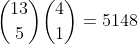
The theory of getting the flush is the following. There are 13 values to choose from, and we want to choose 5 different values. Then, since all of the cards must be the same suit, it must be that we multiply it by 4 choose 1 since there are a total of four suits and pick one suit. Therefore, the total number of ways to get a flush is the following:
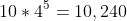
The odds of getting a straight is the following. There are 10 ways to get a sequence (let T stand for 10). A2345, 23456,34567,45678,56789,6789T, 789TJ, 89TJQ, 9TJQK,TJQKA. Next, there are 4 ways to choose the card 5 times each. Therefore, total straight count is the following:
Next, we have to count the number of straight flushes so that we can subtract the count from both of the previous numbers that have been computed. The number of straight flushes will be to multiply 10 (the number of sequences) by four (the total number of suits.)
Therefore, the total number of straights will be 10,240-40 =10,200. The total number of flushes will be 5148-40=5,108. To get the odds divide each number by the total ways to choose 5 cards from a 52 card deck.
The code to simulate each are the following:
import random

class Card():
    def __init__(self, value, suit):
        self._value = value
        self._suit = suit

    def value(self):
        return self._value

    def suit(self):
        return self._suit

    def __str__(self):
        return "" + self._suit + str(self._value)

def create_deck():
    deck = []
    suit = ["H", "D", "S", "C"]

    for i in range(13):
        for j in range(4):
            deck.append(Card(i, suit[j]))

    return deck

def shuffle_deck(deck):
    random.shuffle(deck)

def draw_hand(deck):
    hand = []

    for i in range(5):
        c = deck.pop()
        hand.append(c)

    return hand

def print_hand(hand):
    print("Hand:", end="")
    for c in hand:
        print(c, "", end="")
    print("")

def has_pair(hand):
    meta_count = 0
    for i in range(5):
        count = 0
        for j in range(i+1, 5):
            if hand[i].value() == hand[j].value():
                count += 1
                continue


        if count == 1:
            meta_count += 1
        elif count == 2:
            return False
        elif count == 3:
            return False

    return meta_count == 1

def three_of_a_kind(hand):
    count_map = {}

    for c in hand:
        if c.value() not in count_map:
            count_map[c.value()] = 1
        else:
            count_map[c.value()] += 1

    has_two_of_a_kind = False
    has_three_of_a_kind = False

    for k in count_map:
        if count_map[k] == 2:
            has_two_of_a_kind = True
        elif count_map[k] == 3:
            has_three_of_a_kind = True

    return has_three_of_a_kind and not has_two_of_a_kind

def four_of_a_kind(hand):
    count_map = {}

    for c in hand:
        if c.value() not in count_map:
            count_map[c.value()] = 1
        else:
            count_map[c.value()] += 1

    has_four_of_a_kind = False

    for k in count_map:
        if count_map[k] == 4:
            return True

    return False

def has_straight(hand):
    # Get the values and sort them
    values = sorted([c.value() for c in hand])

    # Check for Ace-High straight explicitly: [0, 9, 10, 11, 12]
    # (Assuming 0 is Ace, 9 is 10, 10 is J, 11 is Q, 12 is K)
    if values == [0, 9, 10, 11, 12]:
        return True

    if len(set(values)) == 5 and (values[-1] - values[0] == 4):
        return True

    return False

def flush(hand):
    s = hand[0].suit()

    for i in range(1, 5):
        if s != hand[i].suit():
            return False

    return True

def main():
    run_count = 100000
    straight_count = 0
    flush_count = 0
    straight_flush_count = 0

    for x in range(run_count):
        deck = create_deck()
        shuffle_deck(deck)
        hand = draw_hand(deck)
        print_hand(hand)

        if flush(hand):
            flush_count += 1

        if has_straight(hand):
            straight_count += 1

        if flush(hand) and has_straight(hand):
            straight_flush_count += 1

    print("Simulation Probability Flush: " + str((flush_count - straight_flush_count)/ 100000.0))
    print("Simulation Probability Straight: " + str((straight_count - straight_flush_count)/ 100000.0))
    print("Simulation Probability Straight Flush: " + str((straight_flush_count)/ 100000.0))

if __name__ == "__main__":
    main()
Final Thoughts
The remaining hands are left as exercises for you to compute the probability by hand, and then simulate in python. In this blog post, you learned how to compute the odds of getting certain hands and simulating the odds in Python.
References
Miller, S. J. (2017). The probability Lifesaver: All the tools you need to understand chance. Princeton University Press.
Logistic population models are one of the most important tools in mathematical biology because they describe how populations grow when resources are limited. Unlike simple exponential growth models, logistic models capture the realistic behavior of populations slowing down as they approach a maximum sustainable size, known as the carrying capacity. From ecology and epidemiology to economics and engineering, these models provide a powerful framework for understanding real-world systems.
In this blog post, you will learn how to develop a mathematical model for logistic population growth step by step. We will begin by exploring the key ideas behind logistic growth and how they differ from exponential models. Then, we will build the governing differential equation and interpret the meaning of each parameter in the model.
Modeling the Problem
Suppose a population only changes based on birth and death rates.
Let B(t) = The number of births per unit population per unit of time t.
Let D(t) = the number of deaths per unit population per unit of time t.
This means the following:
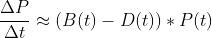
This means the change in population is the following:
which means that
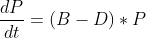
The error should approach zero as delta t approaches 0, which yields the following differential equation:
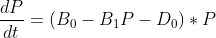
Now, suppose that the birthrate is a linear decreasing function of the population size, so B = B_0 – B_1*P where B_0 and B_1 are constants and greater than zero. Also suppose the death rate is constant, then the following holds:
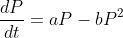
Therefore, this results in the following equation where a = B_0 – D_0 and b = B_1
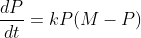
It is useful to rewrite as the following where k=b and M = a/b. Here M is the limiting population.
Solving for a Solution
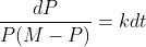
The equation is separable, so it is separated as follows:
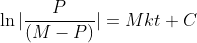
Now, we just integrate both sides. Also, note: for the left hand side, one must use partial fractions to integrate. You should get the following result:
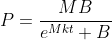
Solving for P, you should get the following the result:
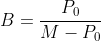
where B is equal to the following when t = 0,
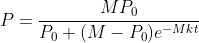
Plugging that value for B, we obtain the final result for the population:
Solving a Logistic Population Problem
Suppose in 1885 the population of a certain country a population of 50 million with a growing rate of 750k per year. Suppose the population in 1940 is 100 million with a growing rate of 1 million per year.
Given the following equation:
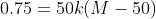
we can solve the following two equations simultaneously:
Doing so will give the values M = 200 and k = 0.0001
Now, let 1940 be t=0. Since M is the limiting population, we have that M = 200 million and P_0 = 100 million
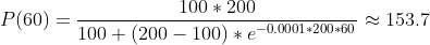
If we want to know what the population will be in the year 2000, we can let t=60, and plug the values into the equation we solved in the previous section. This becomes
Therefore, the population is approximately 153.7 million people in the year 2000.
Final Thoughts
In this blog post, you learned how to model logistic populations, and you learned how to solve problems using the derived equation.
A system of differential equations contain two or more equations that are related by two dependent variables that share a single common independent variable like t for time. Applications of systems of differential equations range from engineering, science, and applied mathematics.
Consider the following system of differential equations:
First, we manually solve for a general solution of the system, then we use MATLAB to come up with a solution.
Solving for a General Solution Manually
The first step is to create a coefficient matrix of the system, then solve for the eigenvalues and associated eigenvectors.
The coefficient matrix for the system is the following:
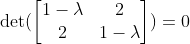
Next, the eigenvalues are solved for, which means solve for the determinant, and set it equal to zero:
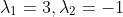
By solving this, you will obtain the following eigenvalues:
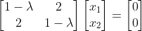
Now that we have the eigenvalues, we can solve for the associated eigenvectors. This can be done by solving the following for each eigenvalue:
Doing so, we obtain the following associated eigenvectors:
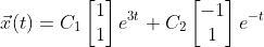
Therefore, the general solution will be the following:
Solving For a General Solution with MATLAB
First, let’s solve for the eigenvectors and eigenvalues using MATLAB. The following code will do that.
% Coefficient matrix
A = [1 2; 2 1];
% Solve for eigenvalues D and eigenvectors V
[V,D] = eig(A);
% Get the first eigenvector and scale
eigV1 = V(:,1) ./ min(V(:,1))
% Get the second eigenvector and scale
eigV2 = V(:,2) ./ min(V(:,2))
x1Vec = -1:0.05:1;
x2Vec = -1:0.05:1;
% x2 = -x1
v1 = -1*x1Vec;
% x2 = x1
v2 = x1Vec;
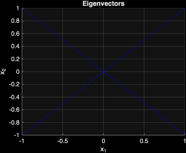
% Plot the eigenvectors
figure;
hold on;
plot(x1Vec,v1,'b');
plot(x1Vec,v2,'b');
xlabel('x_{1}');
ylabel('x_{2}');
grid on;
title('Eigenvectors');
% put the axes on the same limits
xlim([-1 1]);
ylim([-1 1]);
The following is the plot that was generated by MATLAB of the two eigenvectors:
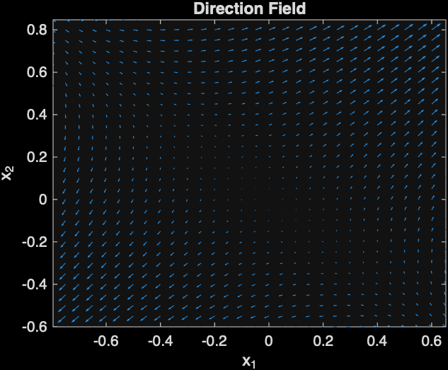
Next, let’s plot the direction field, which will show the direction of solution curves with respect to time.
The following MATLAB code will do that:
[x1, x2] = meshgrid(x1Vec,x2Vec);
% Compute the direction field at the grid of points
x1dot = x1 + 2*x2;
x2dot = 2*x1 + x2;

% The quiver command can be used to plot the direction field
figure;
quiver(x1,x2,x1dot, x2dot);
xlabel('x_{1}');
ylabel('x_{2}');
title('Direction Field');
xlim([-1 1]);
ylim([-1 1]);
The following direction field was generated by MATLAB:
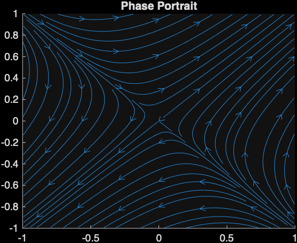
Next, a phase portrait will be generated with MATLAB, which will show the relationship between x1 and x2 with respect to time. The arrows shows the point on a particular solution curve with respect to time.
This image indicates that the point (0,0) is a saddle point. Also, you can tell that the graph will be a saddle because the eigenvalues are both real and one is positive and the other is negative.
Final Words
You saw an example of solving a system of differential equations, and you learned how to solve it using MATLAB.
Euler’s method is used for numerical approximation of a solution to a differential equation that can’t be solved for an explicit solution using elementary methods, such as substitution for homogeneous equations or Bernoulli equations (Henry Edwards et al., 2022). Katherine Johnson used Euler’s method to solve real-world problems at NASA (Meyers, 2017). Personally, I disagree with her claim that math is either absolutely right or absolutely wrong, though.
The algorithm for Euler’s method is to first pick an initial point
of the particular solution you want to compute (Henry Edwards et al., 2022). Then, one chooses a horizontal step-size h, which is the horizontal distance between the approximated points of the solution. The formula to calculate the (n+1)-th point is the following (Henry Edwards et al., 2022):
where
One must be careful when using Euler’s method because there is a local error when moving away from the initial point, which is a vertical distance from the approximated point to the actual point of the particular solution curve (Henry Edwards et al., 2022). As one moves further from the initial point, the error accumulates, and it is called cumulative error (Henry Edwards et al., 2022). The remedy for this is to choose a sufficiently small step size, which will reduce the error (Henry Edwards et al., 2022). However, there is typically a tradeoff when picking h because when h is too small, it may take thousands of years to compute even with a computer (Henry Edwards et al., 2022).
Katherine Johnson was an African American applied mathematician who worked at NASA (Meyers, 2017). She suggested to use Euler’s method to solve differential equations related to the trajectory of astronaut John Glenn’s space capsule. Despite the method being “ancient”, as described by one of her male colleagues, she rebutted that “it works numerically” (Meyers, 2017).
When Katherine Johnson claims “math: you’re either right or wrong — and that I liked about it” (National Geographic, 2021, 0:45) , I tend to disagree. I disagree because sometimes oversimplified models can enable one to capture important insights into the problem. For example, the Lotka-Volterra predator-prey model allows one to see that predator-prey populations oscillate; however, the models typically do not allow one to actually predict the populations in nature (Chasnov, 2022; Clark & Neuhauser, 2022). This is a case in mathematics where it is possible to be partially correct.
In conclusion, Euler’s method is an old yet effective way to numerically approximate solutions to differential equations. It has been used to solve real-world problems in NASA by applied mathematicians like Katherine Johnson to calculate trajectories of a space capsule. Also, despite Katherine Johnson’s claim that one is either right or wrong in math, I think that it is possible to be partially correct in math in the case of oversimplified models that allow one to gain further insights into problems like the Lotka-Volterra predator-prey model.
Using MATLAB to Obtain a Numerical Approximation of a Solution
Next, MATLAB will be used to solve the following differential equation:
with initial condition y(0) = -3.
The following is the MATLAB code to do so:
% Euler's Method for solving:
% y' = x + (1/5)y
% y(0) = -3

clc;
clear;

% Step size
h = 1;

% Interval
x0 = 0;
xn = 5;

% Initial condition
y0 = -3;

% Number of steps
n = (xn - x0)/h;

% Arrays to store values
x = zeros(1, n+1);
y = zeros(1, n+1);

% Initial values
x(1) = x0;
y(1) = y0;

% Euler's Method loop
for i = 1:n
    x(i+1) = x(i) + h;
    y(i+1) = y(i) + h * ( x(i) + (1/5)*y(i) );
end

% Display results
disp('   x          y');
disp([x' y']);

% Plot the approximation
plot(x, y, '-', 'LineWidth', 1.5);
xlabel('x');
ylabel('y');
title('Euler Method Approximation');
grid on;
Clark, A. T., & Neuhauser, C. (2018). Harnessing uncertainty to approximate mechanistic models of interspecific interactions. Theoretical Population Biology, 123, 35–44. https://doi.org/10.1016/j.tpb.2018.05.002
Henry Edwards, C., Penney, D. E., & Calvis., D. (2022). Differential Equations and Boundary Value Problems: Computing and Modeling (6th Edition).